The community structure itself can tell us a lot about the network. If these communities are indeed functional modules in the cell, the largest community should tell us which function in the cell requires the largest number of proteins, and therefore the most resources and energy. More importantly for us, it can also tell us which of the functional modules are most influential on the rest of the cell.
To describe how influential a community is, it is helpful to the abstract the PPI network one step further. We view the communities themselves as individual nodes in a broader community network. This network should not be binary; the communities vary so dramatically in size and are so highly connected that we would lose too much information about the network topology if we were to treat all edges the same. The network should instead be weighted depending on how connected communities are.
The Jaccard Coefficient
To quantify the closeness of adjacent communities, we used the link-based Jaccard coefficient proposed in (1). The Jaccard coefficient, more broadly, is a measure of similarity on sets. For sets \(A\) and \(B\), the Jaccard coefficient, \(J(A,B)\), compares their intersection and union, \[ J(A,B) = \frac{\lvert A \cap B \rvert}{\lvert A \cup B \rvert},\] and is mamximum (\(J = 1\)) when the sets coincide. In the context of networks we have two clear notions of sets: sets of nodes and sets of edges. Since we are interested in the interactions between proteins, and these interactions gives our network its complicated topology, we decided to implement an edge-based Jaccard coefficient. We define the Jaccard coefficient of two communities \(C_A\) and \(C_B\) with sets of nodes \(A\) and \(B\) as \[ \mathfrak{J}(C_A,C_B) = \frac{\text{InterEdges}(A,B)}{\text{NumEdges}(A \cup B)}, \] where \(\text{InterEdges}(A,B)\) is the number of edges with one end in \(C_A\) and the other in \(C_B\), and \(\text{NumEdges}(A \cup B)\) is the number of edges with a least one end in either \(C_A\) or \(C_B\).
This is implemented in the function jdistance(A,B) in Listing 1. In practice, \(\text{InterEdges}(A,B)\) is the cut size of \(C_A\) and \(C_B\), which is easy to calculate in networkx usign the edge_boundary function. We can find \(\text{InterEdges}(A,B)\) by summing over the degrees of nodes in \(A\) and \(B\), and removing edges between nodes in \(A\) and \(B\) which are counted twice (i.e. intraedges).
Listing 1: Function calculating the Jaccard Distance Between Communities
def num_edges(A,B): num =0 intraedge =0for node in A + B: num += G.degree[node]for node1 in A + B:if node == node1:continueelse: intraedge += G.number_of_edges(node,node1)return num - intraedge/2def interedges(A,B): cut = [*nx.edge_boundary(G,A,B)]def jdistance(A,B):return interedges(A,B)/(num_edges(A, B))
A Note on Other Distance Measures
We also considered using other measures for the distance between communities, for example, the ‘average restricted distance’ discussed in (2), which averages over the shortest path lengths between all nodes from two communities, where each edge in the path is required to be within the subgraph induced by the two communities. We decided to use Jaccard coefficient over this because we thought that in a densely connected network such as ours, privileging shortest paths could lead to losses in information, and is not in harmony with our diffusion-based philosophy of ‘considering all paths’. (Both methods, at any rate, returned similar results.)
Listing 2: Function calculating the Restricted Distance Between Communities
def distance(A,B): distances = [] nodes = A + B AB = G.subgraph(nodes)ifnot nx.is_connected(AB):return0for nodeA in A:for nodeB in B: distances.append(nx.shortest_path_length(AB,nodeA,nodeB))return np.average(distances)
Pruning Communities
It is impossible to visualise all 580 communities at the same time in a meaningful way, so we prune the network before plotting. In fact, there are 250 communities with only 1 protein. The reason why WalkTrap has produced so many single-node communities is unclear and should be investigated; perhaps these proteins sit between densely clustered areas in the network.
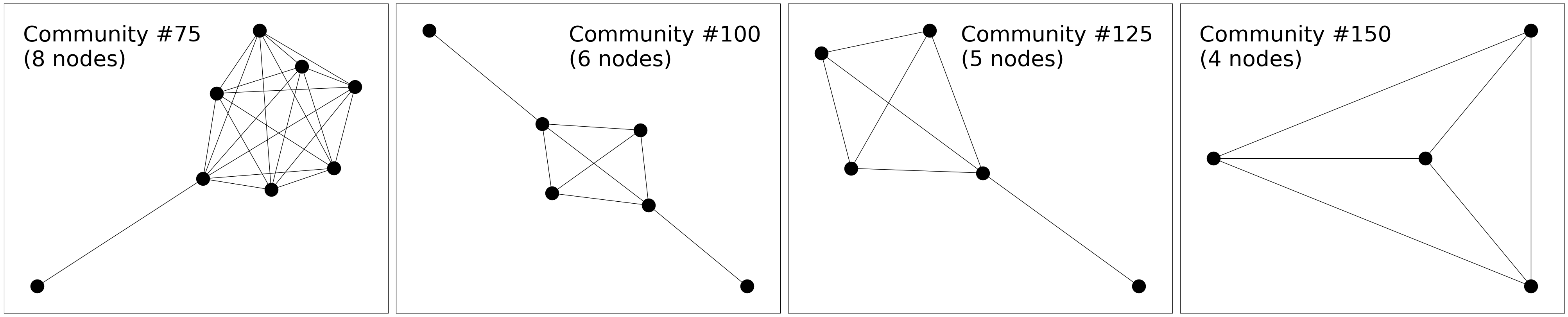
Arbitrarily, we choose to prune the network of communities with 10 or fewer members; leaving 56 communities. A sample of the communities which we removed are shown below (community #75, #100, #125 and #150). They are highly connected clique-like networks, and are therefore likely complexes of proteins (3) rather than larger functional groups, which we are more interested in, so their removal is justified.
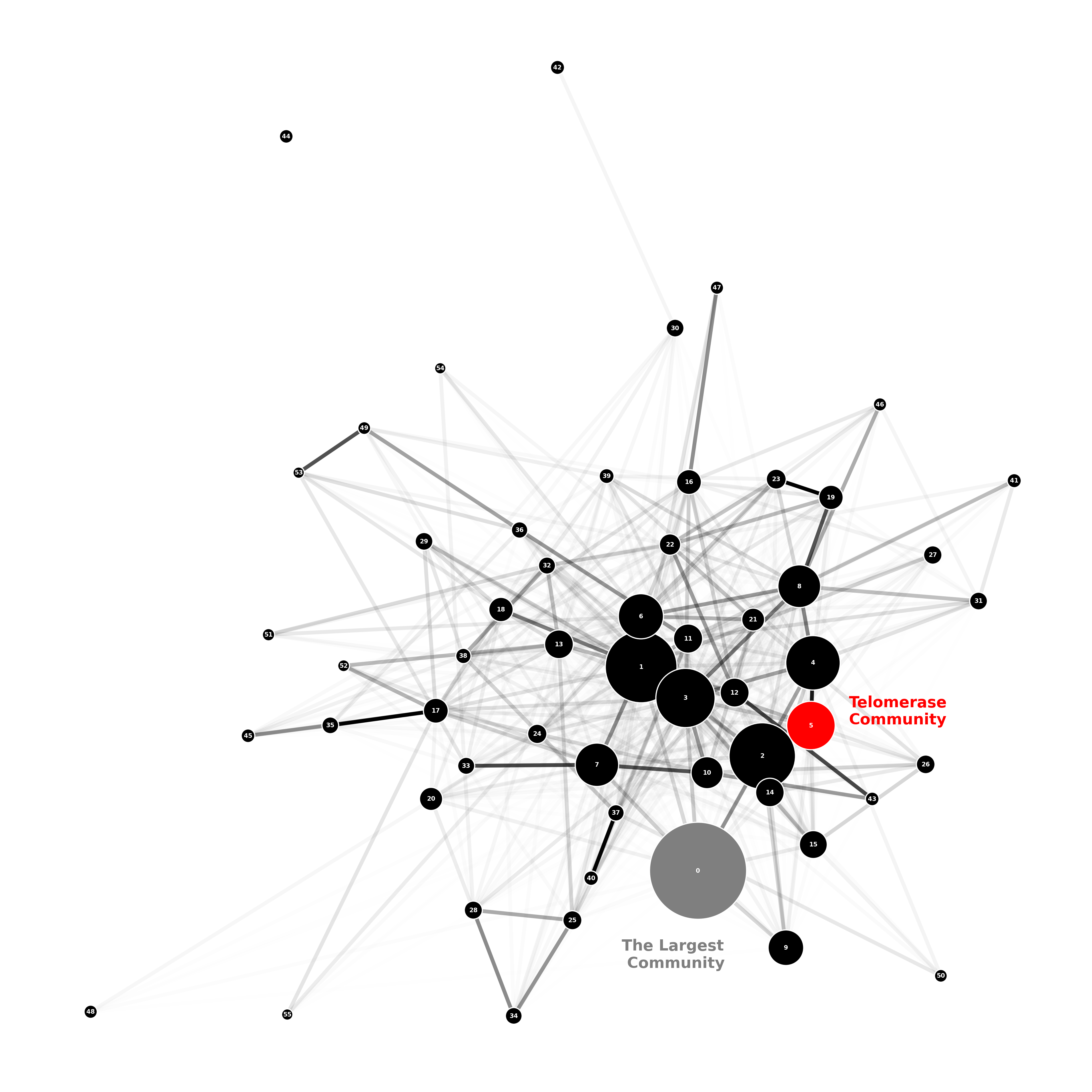
This allows us to visualise the connections between the communities in Figure 1. The largest community, 0, and the telomerase community, 5, are labelled. The transparency of the edges is set by alpha = np.min([15*d[“weight”], 1]), where d[“weight”] is the Jaccard distance between communities. Darker edges therefore represent stronger connections. The size of nodes in the network is determined by the number of proteins in each community and is set by the line: node_sizes = [len(walktrapG[i])*20 for i in range(0,len(walktrapG)) if len(walktrapG[i]) > 10].
Code
#~~~~~~~~~~~~~~~~~~~~~~~~~~~~~~~~~~~~~# Packages and Modules#~~~~~~~~~~~~~~~~~~~~~~~~~~~~~~~~~~~~~import networkx as nximport numpy as npimport scipy as spimport igraph as igimport matplotlib.pyplot as pltimport math from networkx.drawing.nx_agraph import graphviz_layoutimport pygraphviztel_id = ['4932.YLR233C', '4932.YLR318W', '4932.YIL009C-A']T ='telomerase'#~~~~~~~~~~~~~~~~~~~~~~~~~~~~~~~~~~~~~# Graph-setup#~~~~~~~~~~~~~~~~~~~~~~~~~~~~~~~~~~~~~G0 = nx.read_weighted_edgelist('Yeast Data/4932.protein.links.v12.0.txt',comments="#",nodetype=str)threshold_score =700for edge in G0.edges: weight =list(G0.get_edge_data(edge[0],edge[1]).values())if(weight[0] <= threshold_score): G0.remove_edge(edge[0],edge[1])largest_cc =max(nx.connected_components(G0),key=len)G = G0.subgraph(largest_cc)# convert to igraph g = ig.Graph.from_networkx(G)#~~~~~~~~~~~~~~~~~~~~~~~~~~~~~~~~~~~~~# Get WalkTrap Communities#~~~~~~~~~~~~~~~~~~~~~~~~~~~~~~~~~~~~~h = g.community_walktrap().as_clustering() # save as VectorClustering objectmem = h.membership # membership vectorwalktrapG = [[] for i inrange(len(h))] # list of lists of community nodesi =0for node in nx.nodes(G): walktrapG[mem[i]].append(node) i +=1walktrapG.sort(key=len, reverse=True)telomerase_community = G.subgraph(walktrapG[5])#~~~~~~~~~~~~~~~~~~~~~~~~~~~~~~~~~~~~~# Conjoin Telomerase into a single entity:#~~~~~~~~~~~~~~~~~~~~~~~~~~~~~~~~~~~~~telomerase_community = nx.contracted_nodes(telomerase_community, tel_id[1], tel_id[0], self_loops=True)telomerase_community = nx.contracted_nodes(telomerase_community, tel_id[1], tel_id[2], self_loops=True)G = nx.contracted_nodes(G,tel_id[1], tel_id[0], self_loops=True)G = nx.contracted_nodes(G,tel_id[1], tel_id[2], self_loops=True)mapping = {'4932.YLR318W':'telomerase'} # relabel node as `telomerase' for ease of referenceG = nx.relabel_nodes(G, mapping)telomerase_community = nx.relabel_nodes(telomerase_community, mapping)for p in tel_id: walktrapG[5].remove(p);walktrapG[5].append(T) # add telomerase############################################################################~~~~~~~~~~~~~~~~~~~~~~~~~~~~~~~~~~~~~# Reading in Jaccard Distance#~~~~~~~~~~~~~~~~~~~~~~~~~~~~~~~~~~~~~file=open('Other Data/jdists.txt', 'r') # read from filelines =file.readlines()jdists_file = [] # Strip newline and split over spacesfor line in lines: L = line.strip().split(' ') jdists_file.append(L)jdists = np.zeros((len(walktrapG), len(walktrapG)))# convert to numbers:for i inrange(0,len(walktrapG)):for j inrange(0,len(walktrapG)): jdists[i,j] =float(jdists_file[i][j])#~~~~~~~~~~~~~~~~~~~~~~~~~~~~~~~~~~~~~# Use Jaccard distance matrix as an adjacency matrix to construct and prune the community network#~~~~~~~~~~~~~~~~~~~~~~~~~~~~~~~~~~~~~community_graph = nx.Graph() # empty graphfor i inrange(0,len(walktrapG)):for j inrange(0,len(walktrapG)): community_graph.add_edge(i, j, weight=jdists[i,j]) # add weights to edges# Remove edges that have 0 weights:for edge in community_graph.edges: weight =list(community_graph.get_edge_data(edge[0],edge[1]).values())if(weight[0] ==0): # Remove edges that have zero weights community_graph.remove_edge(edge[0],edge[1])# Remove communities that are small (likely complexes):remove_complexes = [i for i inrange(0,len(walktrapG)) iflen(walktrapG[i]) <=10]for i in remove_complexes: community_graph.remove_node(i)############################################################################~~~~~~~~~~~~~~~~~~~~~~~~~~~~~~~~~~~~~# Plot the network:#~~~~~~~~~~~~~~~~~~~~~~~~~~~~~~~~~~~~~#~~~~~~~~~~~~~~~~~~~~~~~~~~~~~~~~~~~~~####### 1. Set-up#~~~~~~~~~~~~~~~~~~~~~~~~~~~~~~~~~~~~~# Get Colormap:color_map = []for node in community_graph:if node ==5: color_map.append('red')elif node ==0: color_map.append('tab:gray')else: color_map.append('black')# Positions of nodes:pos = nx.spring_layout(community_graph, seed=60)# Side of nodes based on number of proteins in each community:node_sizes = [len(walktrapG[i])*20for i inrange(0,len(walktrapG)) iflen(walktrapG[i]) >10]#~~~~~~~~~~~~~~~~~~~~~~~~~~~~~~~~~~~~~####### 2. Plot Figure#~~~~~~~~~~~~~~~~~~~~~~~~~~~~~~~~~~~~~fig = plt.figure(figsize=(20,20))# Draw nodesnx.draw_networkx_nodes(community_graph, pos, node_color=color_map, node_size=node_sizes, edgecolors='w', linewidths=1.5)# Label nodesnx.draw_networkx_labels(community_graph, pos, font_size=8, font_family="sans-serif", font_color='w', font_weight='bold')# Draw edges: # loop through each edge and plot individually, changing the transparency of the edge depending on the strength of connection[nx.draw_networkx_edges(community_graph, pos,edgelist=[(u,v)], alpha=(np.min([15*d["weight"], 1])),width=5) for (u, v, d) in community_graph.edges(data=True)];# Label telomerase community:plt.annotate("Telomerase\nCommunity", xy=(0.78,0.335), xycoords='axes fraction', weight='bold', size=20, color='r')plt.annotate("The Largest\n Community", xy=(0.57,0.11), xycoords='axes fraction', weight='bold', size=20, color='tab:gray')ax = plt.gca()plt.axis("off")plt.tight_layout()plt.show()
Figure 1: Jaccard Distance Community Visualisation
Important Communities and a Comment on Functional Groups.
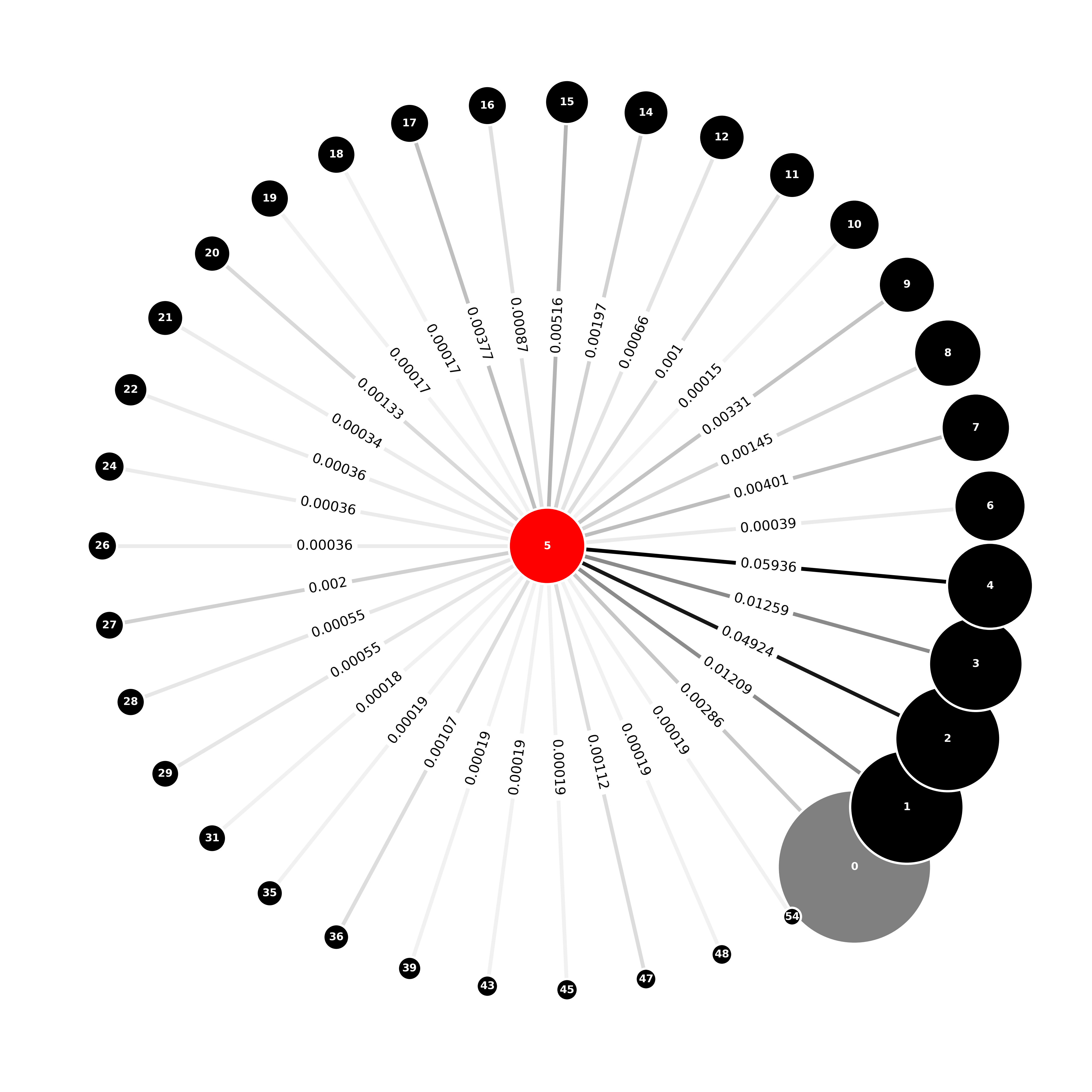
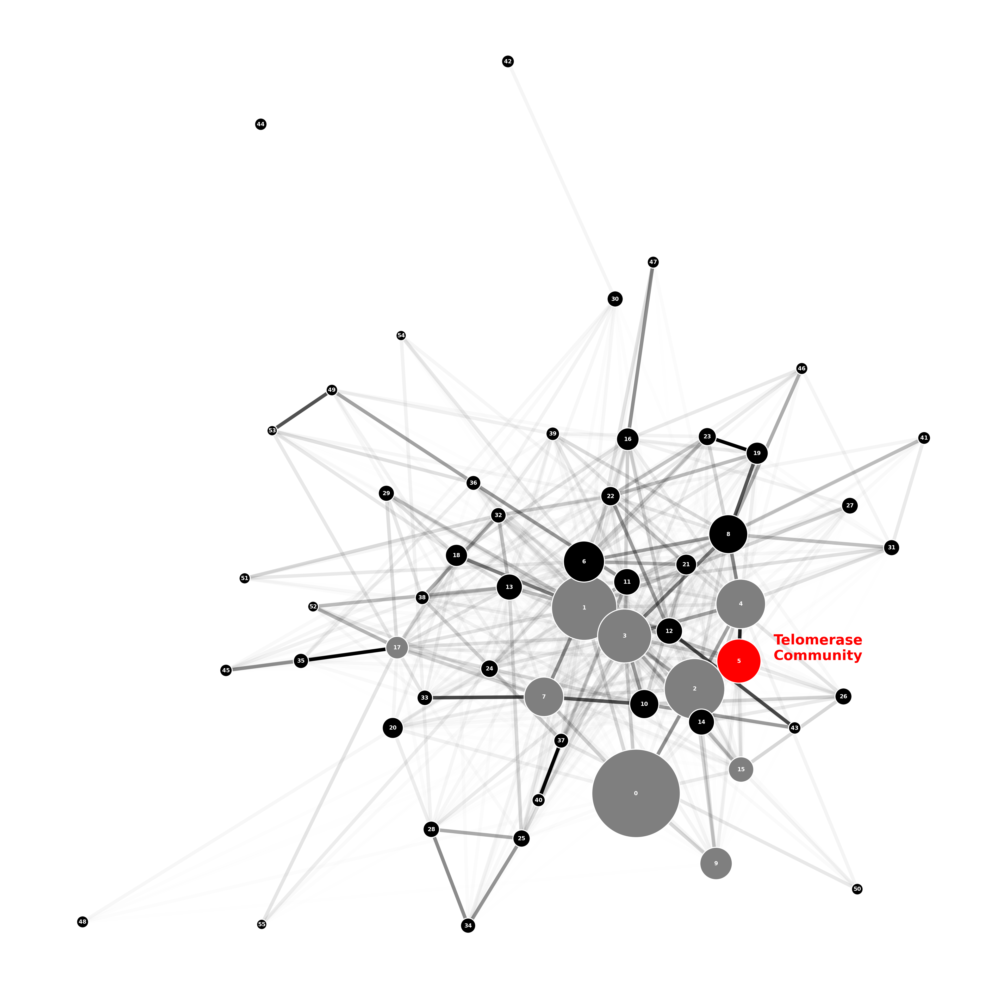
An ego_graph of the communities joined to the telomerase community is shown below in Figure 2, with edges labelled by the Jaccard distance. The nine closest communities to the telomerase community are communities: 0, 1, 2, 3, 4, 7, 9, 15 and 17 which are highlighted in grey in Figure 3; we will use these, shortly, in our discussion of diffusion distance.
Code
#~~~~~~~~~~~~~~~~~~~~~~~~~~~~~~~~~~~~~# Packages and Modules#~~~~~~~~~~~~~~~~~~~~~~~~~~~~~~~~~~~~~import networkx as nximport numpy as npimport scipy as spimport igraph as igimport matplotlib.pyplot as pltimport math from networkx.drawing.nx_agraph import graphviz_layoutimport pygraphviztel_id = ['4932.YLR233C', '4932.YLR318W', '4932.YIL009C-A']T ='telomerase'#~~~~~~~~~~~~~~~~~~~~~~~~~~~~~~~~~~~~~# Graph-setup#~~~~~~~~~~~~~~~~~~~~~~~~~~~~~~~~~~~~~G0 = nx.read_weighted_edgelist('Yeast Data/4932.protein.links.v12.0.txt',comments="#",nodetype=str)threshold_score =700for edge in G0.edges: weight =list(G0.get_edge_data(edge[0],edge[1]).values())if(weight[0] <= threshold_score): G0.remove_edge(edge[0],edge[1])largest_cc =max(nx.connected_components(G0),key=len)G = G0.subgraph(largest_cc)# convert to igraph g = ig.Graph.from_networkx(G)#~~~~~~~~~~~~~~~~~~~~~~~~~~~~~~~~~~~~~# Get WalkTrap Communities#~~~~~~~~~~~~~~~~~~~~~~~~~~~~~~~~~~~~~h = g.community_walktrap().as_clustering() # save as VectorClustering objectmem = h.membership # membership vectorwalktrapG = [[] for i inrange(len(h))] # list of lists of community nodesi =0for node in nx.nodes(G): walktrapG[mem[i]].append(node) i +=1walktrapG.sort(key=len, reverse=True)telomerase_community = G.subgraph(walktrapG[5])#~~~~~~~~~~~~~~~~~~~~~~~~~~~~~~~~~~~~~# Conjoin Telomerase into a single entity:#~~~~~~~~~~~~~~~~~~~~~~~~~~~~~~~~~~~~~telomerase_community = nx.contracted_nodes(telomerase_community, tel_id[1], tel_id[0], self_loops=True)telomerase_community = nx.contracted_nodes(telomerase_community, tel_id[1], tel_id[2], self_loops=True)G = nx.contracted_nodes(G,tel_id[1], tel_id[0], self_loops=True)G = nx.contracted_nodes(G,tel_id[1], tel_id[2], self_loops=True)mapping = {'4932.YLR318W':'telomerase'} # relabel node as `telomerase' for ease of referenceG = nx.relabel_nodes(G, mapping)telomerase_community = nx.relabel_nodes(telomerase_community, mapping)for p in tel_id: walktrapG[5].remove(p);walktrapG[5].append(T) # add telomerase############################################################################~~~~~~~~~~~~~~~~~~~~~~~~~~~~~~~~~~~~~# Reading in Jaccard Distance#~~~~~~~~~~~~~~~~~~~~~~~~~~~~~~~~~~~~~file=open('Other Data/jdists.txt', 'r') # read from filelines =file.readlines()jdists_file = [] # Strip newline and split over spacesfor line in lines: L = line.strip().split(' ') jdists_file.append(L)jdists = np.zeros((len(walktrapG), len(walktrapG)))# convert to numbers:for i inrange(0,len(walktrapG)):for j inrange(0,len(walktrapG)): jdists[i,j] =float(jdists_file[i][j])#~~~~~~~~~~~~~~~~~~~~~~~~~~~~~~~~~~~~~# Use Jaccard distance matrix as an adjacency matrix to construct and prune the community network#~~~~~~~~~~~~~~~~~~~~~~~~~~~~~~~~~~~~~community_graph = nx.Graph() # empty graphfor i inrange(0,len(walktrapG)):for j inrange(0,len(walktrapG)): community_graph.add_edge(i, j, weight=jdists[i,j]) # add weights to edges# Remove edges that have 0 weights:for edge in community_graph.edges: weight =list(community_graph.get_edge_data(edge[0],edge[1]).values())if(weight[0] ==0): # Remove edges that have zero weights community_graph.remove_edge(edge[0],edge[1])# Remove communities that are small (likely complexes):remove_complexes = [i for i inrange(0,len(walktrapG)) iflen(walktrapG[i]) <=10]for i in remove_complexes: community_graph.remove_node(i)############################################################################~~~~~~~~~~~~~~~~~~~~~~~~~~~~~~~~~~~~~# Plot the network:#~~~~~~~~~~~~~~~~~~~~~~~~~~~~~~~~~~~~~around_5 = nx.generators.ego_graph(community_graph, 5, radius=1)#~~~~~~~~~~~~~~~~~~~~~~~~~~~~~~~~~~~~~####### 1. Set-up#~~~~~~~~~~~~~~~~~~~~~~~~~~~~~~~~~~~~~# Get Colormap:color_map = []for node in around_5:if node ==5: color_map.append('red')elif node ==0: color_map.append('tab:gray')else: color_map.append('black')#~~~~~~~~~~~~~~~~~~~~~~~~~~~~~~~~~~~~~~~~~~~~~~~~~~~~~~~~~~~~~~~~edges = around_5.edges()for e in edges:if e[0] !=5and e[1] !=5: around_5.remove_edge(e[0], e[1])node_sizes = [len(walktrapG[i])*50for i in around_5.nodes() iflen(walktrapG[i]) >10]#~~~~~~~~~~~~~~~~~~~~~~~~~~~~~~~~~~~~~~~~~~~~~~~~~~~~~~~~~~~~~~~~# get color-map and set-up: color_map = []for node in around_5:if node ==5: color_map.append('red')elif node ==0: color_map.append('grey')else: color_map.append('black')pos_5 = graphviz_layout(around_5, 'twopi')#~~~~~~~~~~~~~~~~~~~~~~~~~~~~~~~~~# plot:fig = plt.figure(figsize=(20,20))# Draw nodesnx.draw_networkx_nodes(around_5, pos_5, node_size=node_sizes, node_color=color_map, edgecolors='w', linewidths=3)# Loop through each edge and plot individually (so we can change alpha each time, depending on degree)max_weight =max([d["weight"] for (u, v, d) in around_5.edges(data=True)])list(around_5.edges(data=True))[2][2][nx.draw_networkx_edges(around_5, pos_5,edgelist=[(u,v)], alpha=(d["weight"]/max_weight)**(1/2), width=5) for (u, v, d) in around_5.edges(data=True)];# Node labelsnx.draw_networkx_labels(around_5, pos_5, font_size=14, font_family="sans serif", font_color='w', font_weight='bold');# Edge labelsedge_labels = nx.get_edge_attributes(around_5, "weight")for e, el inzip(edge_labels, edge_labels.values()): edge_labels[e] = np.round(el, 5) # round weights for easenx.draw_networkx_edge_labels(around_5, pos_5, edge_labels, font_size=18)#~~~~~~~~~~~~~~~~~~~~~~~~~~~~~~~~~ax = plt.gca()ax.margins(0.08)plt.axis("off")plt.tight_layout()plt.show()
Figure 2: Jaccard Distance Around the Telomerase Community
Code
#~~~~~~~~~~~~~~~~~~~~~~~~~~~~~~~~~~~~~# Packages and Modules#~~~~~~~~~~~~~~~~~~~~~~~~~~~~~~~~~~~~~import networkx as nximport numpy as npimport scipy as spimport igraph as igimport matplotlib.pyplot as pltimport math from networkx.drawing.nx_agraph import graphviz_layoutimport pygraphviztel_id = ['4932.YLR233C', '4932.YLR318W', '4932.YIL009C-A']T ='telomerase'#~~~~~~~~~~~~~~~~~~~~~~~~~~~~~~~~~~~~~# Graph-setup#~~~~~~~~~~~~~~~~~~~~~~~~~~~~~~~~~~~~~G0 = nx.read_weighted_edgelist('Yeast Data/4932.protein.links.v12.0.txt',comments="#",nodetype=str)threshold_score =700for edge in G0.edges: weight =list(G0.get_edge_data(edge[0],edge[1]).values())if(weight[0] <= threshold_score): G0.remove_edge(edge[0],edge[1])largest_cc =max(nx.connected_components(G0),key=len)G = G0.subgraph(largest_cc)# convert to igraph g = ig.Graph.from_networkx(G)#~~~~~~~~~~~~~~~~~~~~~~~~~~~~~~~~~~~~~# Get WalkTrap Communities#~~~~~~~~~~~~~~~~~~~~~~~~~~~~~~~~~~~~~h = g.community_walktrap().as_clustering() # save as VectorClustering objectmem = h.membership # membership vectorwalktrapG = [[] for i inrange(len(h))] # list of lists of community nodesi =0for node in nx.nodes(G): walktrapG[mem[i]].append(node) i +=1walktrapG.sort(key=len, reverse=True)telomerase_community = G.subgraph(walktrapG[5])#~~~~~~~~~~~~~~~~~~~~~~~~~~~~~~~~~~~~~# Conjoin Telomerase into a single entity:#~~~~~~~~~~~~~~~~~~~~~~~~~~~~~~~~~~~~~telomerase_community = nx.contracted_nodes(telomerase_community, tel_id[1], tel_id[0], self_loops=True)telomerase_community = nx.contracted_nodes(telomerase_community, tel_id[1], tel_id[2], self_loops=True)G = nx.contracted_nodes(G,tel_id[1], tel_id[0], self_loops=True)G = nx.contracted_nodes(G,tel_id[1], tel_id[2], self_loops=True)mapping = {'4932.YLR318W':'telomerase'} # relabel node as `telomerase' for ease of referenceG = nx.relabel_nodes(G, mapping)telomerase_community = nx.relabel_nodes(telomerase_community, mapping)for p in tel_id: walktrapG[5].remove(p);walktrapG[5].append(T) # add telomerase############################################################################~~~~~~~~~~~~~~~~~~~~~~~~~~~~~~~~~~~~~# Reading in Jaccard Distance#~~~~~~~~~~~~~~~~~~~~~~~~~~~~~~~~~~~~~file=open('Other Data/jdists.txt', 'r') # read from filelines =file.readlines()jdists_file = [] # Strip newline and split over spacesfor line in lines: L = line.strip().split(' ') jdists_file.append(L)jdists = np.zeros((len(walktrapG), len(walktrapG)))# convert to numbers:for i inrange(0,len(walktrapG)):for j inrange(0,len(walktrapG)): jdists[i,j] =float(jdists_file[i][j])#~~~~~~~~~~~~~~~~~~~~~~~~~~~~~~~~~~~~~# Use Jaccard distance matrix as an adjacency matrix to construct and prune the community network#~~~~~~~~~~~~~~~~~~~~~~~~~~~~~~~~~~~~~community_graph = nx.Graph() # empty graphfor i inrange(0,len(walktrapG)):for j inrange(0,len(walktrapG)): community_graph.add_edge(i, j, weight=jdists[i,j]) # add weights to edges# Remove edges that have 0 weights:for edge in community_graph.edges: weight =list(community_graph.get_edge_data(edge[0],edge[1]).values())if(weight[0] ==0): # Remove edges that have zero weights community_graph.remove_edge(edge[0],edge[1])# Remove communities that are small (likely complexes):remove_complexes = [i for i inrange(0,len(walktrapG)) iflen(walktrapG[i]) <=10]for i in remove_complexes: community_graph.remove_node(i)############################################################################~~~~~~~~~~~~~~~~~~~~~~~~~~~~~~~~~~~~~# Plot the network:#~~~~~~~~~~~~~~~~~~~~~~~~~~~~~~~~~~~~~#~~~~~~~~~~~~~~~~~~~~~~~~~~~~~~~~~~~~~####### 1. Set-up#~~~~~~~~~~~~~~~~~~~~~~~~~~~~~~~~~~~~~# Get Colormap:closest9 = [0,1,2,3,4,7,9,15,17] # closest 9 to community 0.color_map = []for node in community_graph:if node ==5: color_map.append('red')elif node in closest9: color_map.append('tab:gray')else: color_map.append('black')# Positions of nodes:pos = nx.spring_layout(community_graph, seed=60)# Side of nodes based on number of proteins in each community:node_sizes = [len(walktrapG[i])*20for i inrange(0,len(walktrapG)) iflen(walktrapG[i]) >10]#~~~~~~~~~~~~~~~~~~~~~~~~~~~~~~~~~~~~~####### 2. Plot Figure#~~~~~~~~~~~~~~~~~~~~~~~~~~~~~~~~~~~~~fig = plt.figure(figsize=(20,20))# Draw nodesnx.draw_networkx_nodes(community_graph, pos, node_color=color_map, node_size=node_sizes, edgecolors='w', linewidths=1.5)# Label nodesnx.draw_networkx_labels(community_graph, pos, font_size=8, font_family="sans-serif", font_color='w', font_weight='bold')# Draw edges: # loop through each edge and plot individually, changing the transparency of the edge depending on the strength of connection[nx.draw_networkx_edges(community_graph, pos,edgelist=[(u,v)], alpha=(np.min([15*d["weight"], 1])),width=5) for (u, v, d) in community_graph.edges(data=True)];# Label telomerase community:plt.annotate("Telomerase\nCommunity", xy=(0.78,0.335), xycoords='axes fraction', weight='bold', size=20, color='r')# plt.annotate("The Largest\n Community", xy=(0.57,0.11), xycoords='axes fraction', weight='bold', size=20, color='tab:gray')ax = plt.gca()plt.axis("off")plt.tight_layout()plt.show()
Figure 3: Jaccard Distance Closest Community Visualisation
Finally, we briefly comment on the functional identity of the five closest communities, 0, 1, 2, 3 and 4, based on their five highest degree-centrality proteins:
Community 0: Proteins: RPS13, RPS5, RPS3, RPS14A, RPL3 Diagnosis: All proteins are ribo-proteins; a community most likely related to the translation of RNA to make proteins.
Community 1: Proteins: PGI1, TKL1, TRP5, ZWF1, ACS1 Diagnosis: All proteins are enzymes; with TKL1 and TRP5 involved in amino acid biosynthesis, and PGT1, ZWF1, and ACS 1 involved in metabolimic pathways; a community that is key to cell survival.
Community 2: Proteins: HHT1, HHF1, HHT2, SPT15, HHF2 Diagnosis: All proteins (other than SPT15) are histones, which wrap around DNA; a community key for DNA and cell survival.
Community 3: Proteins: HSP82, HSC82, KAR2, YDJ1, HSP104 Diagnosis: All proteins (other than HSP104) have chaperone activity, helping with protein folding; HSP104 is still relevant as it is involved in the heat shock and stress response; knock-out might not be lethal, but could change the phenotype of the cell.
Community 4: Proteins: CDC28, CDC20, CDC5, MAD2, CLB2 Diagnosis: All proteins are cell cycle regulators, or their activity is dependent on the cell cycle; most likely related to meiosis.
These communities play key roles in the survival of the cell. It is therefore extremely important that our protein knock-out is localised to proteins nearest to the telomerase community.
Adali S, Lu X, Magdon-Ismail M. Deconstructing centrality: Thinking locally and ranking globally in networks. In: Proceedings of the 2013 IEEE/ACM international conference on advances in social networks analysis and mining [Internet]. New York, NY, USA: Association for Computing Machinery; 2013. p. 418–25. (ASONAM ’13). Available from: 10.1145/2492517.2492531
3.
Chen B, Fan W, Liu J, Wu FX. Identifying protein complexes and functional modules—from static PPI networks to dynamic PPI networks. Briefings in Bioinformatics [Internet]. 2013 Jun;15(2):177–94. Available from: https://doi.org/10.1093/bib/bbt039